Sensitivity Analysis
Objective Function Coefficient Ranges
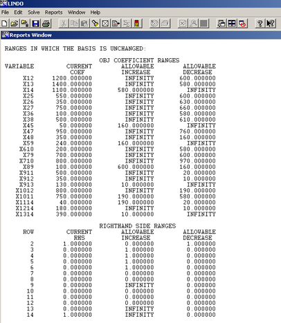
For each objective function coefficient, the range is given in the OBJECTIVE COEFFICIENT RANGES portion of the LINDO output.
The ALLOWABLE INCREASE (AI) section indicates:
· The amount by which an objective function coefficient can be increased with the current basis remaining optimal. Similarly,
The ALLOWABLE DECREASE (AD) section indicates:
· The amount by which an objective function coefficient can be decreased with the current basis remaining optimal.
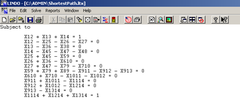
For the Student Night Out problem let cij be the Objective Function Coefficient for xij. (i is the start node, j is the finish node for that arc)
If c14 changed, the current remain optimal if:
1100 – AD ≤ c14 ≤ 1100 + AI
1100 – ∞ ≤ c14 ≤ 1100 + 580
– ∞ ≤ c14 ≤ 1680
This is known as allowable range for c14. If cij remains in the allowable range then the values of the decision variables remain unchanged, although the optimal z – value may change.
The ALLOWABLE INCREASE (AI) section indicates:
· The amount by which an objective function coefficient can be increased with the current basis remaining optimal. Similarly,
The ALLOWABLE DECREASE (AD) section indicates:
· The amount by which an objective function coefficient can be decreased with the current basis remaining optimal.
For the Student Night Out problem let cij be the Objective Function Coefficient for xij. (i is the start node, j is the finish node for that arc)
If c14 changed, the current remain optimal if:
1100 – AD ≤ c14 ≤ 1100 + AI
1100 – ∞ ≤ c14 ≤ 1100 + 580
– ∞ ≤ c14 ≤ 1680
This is known as allowable range for c14. If cij remains in the allowable range then the values of the decision variables remain unchanged, although the optimal z – value may change.
Reduced Costs and Sensitivity Analysis
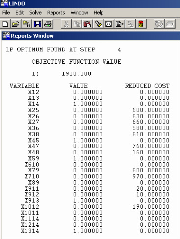
The REDUCED COST portion of the LINDO output indicates:
· How changing the objective function coefficient for a nonbasic variable will change the LP’s optimal solution.
· For any nonbasic variable xk, the reduced cost is the amount by which the objective function coefficient of xk must be improved before the LP will have an optimal solution in which xk is a basic variable.
· If the objective function coefficient of a nonbasic variable xk is improved by its reduced cost, then the LP will have alternative optimal solutions—at least one in which xk is a basic variable, and at least one in which xk is not a basic variable.
· If the objective function coefficient of a nonbasic variable xk is improved by more than its reduced cost, then (barring degeneracy) any optimal solution to the LP will have xk as a basic variable and xk > 0.
For the Student Night Out problem the basic variables associated with the optimal solution are x14, x45, x59, x913, x1314
The nonbasic variable x25 has a reduced cost of 600 this implies that if the objective function coefficient of x25 is decreased (in this case, the distance between node 2 and node 5) by exactly 600, then there will be alternative optimal solutions. In at least one of these optimal solutions x25 will be a basic variable. If the distance of x25 is decreased by more than 600, then any optimal solution to the LP will have x25 as a basic variable (with x25 > 0).
Right-Hand Side Ranges
One can determine (at least for a two-variable problem) the range of values for a right-hand side within which the current basis remains optimal. This information is given in the RIGHTHAND SIDE RANGES section of the LINDO output.
For this LP the ranges can not be changed since the first and the last node are the only ones that can be equal to 1, the others have to be equal to 0.
For this LP the ranges can not be changed since the first and the last node are the only ones that can be equal to 1, the others have to be equal to 0.
Shadow Prices and Dual Prices
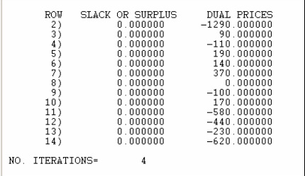
· The shadow price of an LP’s ith constraint can be defined to be the amount by which the optimal z value of the LP is improved if the right-hand side is decreased by one unit (assuming this change leaves the current basis optimal).
· If, after a change in a constraint’s right-hand side, the current basis is no longer optimal, then the shadow prices of all constraints may change.
· The shadow price for each constraint is found in the DUAL PRICES section of the LINDO output.
· If we increase the right hand side of the ith constraint by an amount bi —a decrease in bi implies that bi < 0—and the new right-hand side value for constraint i remains within the allowable range for the right-hand side given in the RIGHTHAND SIDE RANGES section of the output, then a new optimal z-value is determined after the righthand side is changed.
Signs of Shadow Prices
· A ≥ constraint will always have a nonpositive shadow price;
· a ≤ constraint will always have a nonnegative shadow price;
· and an equality constraint may have a positive, negative, or zero shadow price.
To see why this is true, observe that adding points to an LP’s feasible region can only improve the optimal z-value or leave it the same. Eliminating points from an LP’s feasible region can only make the optimal z-value worse or leave it the same.
